Logarithmic timing
This file was created in October 2011 by
Hermann Gottschewski. Ask your questions to
gottschewski@fusehime.c.u-tokyo.ac.jp)
One of the most common features of musical
timing is to slow down (ritardando) and go back
to the main tempo (a tempo) at a structurally
meaningful spot such as the entry of a new theme. The sudden tempo change that
happens in this case is often mediated by a certain tempo ratio. Using a tempo
ratio means that the musical pulses don not stop
with the end of the ritardando, but they switch
from one metrical level to another. If, for instance, the tempo of the eighth
notes slows down to the half tempo and the original tempo is reestablished
(i.e. the tempo doubles suddenly), the eighth
note pulse will continue on the quarter note level after the a tempo.
Normally students are advised to use this
feature of timing not to often, because a ritardando interrupts the flow of musical time. Analysis of musical timing in
romantic music, however, has shown that a regular slowing down and frequent reestablishment of time (for example at
the beginning of every bar) does not necessarily interrupt the musical flow.
(See for example Hermann Gottschewski: Die Interpretation als Kunstwerk, p. 298.) The reason for this phenomenon is that the process of
timing as a whole (i.e. slowing down and reestablishment of the original tempo)
is perceived as one musical “happening”, and its repetition can establish a new
musical pulse that bears the musical flow.
The most appropriate theoretical model of
this process can be found in the logarithmic scale with the base 2.[1]
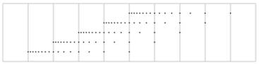
The picture below shows how in a 4/4 meter the eighth notes slow down within
the time of one bar, and in the following bar the tempo is doubled. Since the
same process is repeated the whole bar pulse remains unchanged.
doubled tempo doubled tempo doubled tempo doubled tempo logarithmic slow down
Application to a
Brahms piece
How this principle can work in a real piece
of music is shown in a synthesized version of the first part of Brahms’
Intermezzo op. 119, no. 4. A mechanical application of this principle, however,
would create a boring effect. So the principle of slowing down two half tempo
and going back to the original tempo is used for one-bar, two-bar or three-bar
sections according to the musical structure, and in the last bar no a tempo is used, so that the slow down continues form half tempo to 1/4
tempo. The whole tempo map of the synthesized part can be shown in a
SKYLINE2-graph (see Die Interpretation als Kunstwerk, p. 246–252). The graph shows a real time axis in the
horizontal dimension and duration of time intervals in the vertical dimension.
That means that growing size of rectangles corresponds to a slow down in tempo.
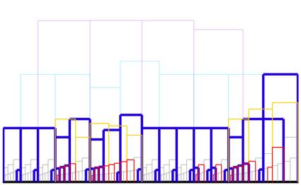
Blue lines in this SKYLINE2-graph show the
time structure of the melody and whole bars, red lines the time structure of
the bass line. Grey lines show the other notes, and lines of other colors show
other metrical relations such as two-bar and three-bar durations.
The time structure was realized in a MIDI
file and then played back with a Yamaha Disklavier at the Musikhochschule
Freiburg in Germany. (I say my thanks to Prof. Sischka and his students for
their kind support of my research.) Dynamics were adjusted at the Disklavier by
ear. In the last step a pedalling was added live by a student and recorded
acoustically.
Audio file without pedalling:
Brahms119_4nopedal.mp3
Audio file with live pedalling:
Brahms119_4livepedal.mp3
In both files the keyboard is played by the
computer, using a mathematically calculated time map (“logarithmic timing”) and
manually adjusted dynamics.
Analysis
Although in this piece a very schematic
pattern of timing is used, the change between one-bar, two-bar and three-bar
units of slow-down allows a certain degree of musical shaping. The bigger fat
blue rectangles, for example, show that the first three bars have the same
length, the fourth bar is shorter and the fifth bar is longer, so that the
fourth and fifth bar together (light blue rectangle) have the same length as
two bars before. That means, that seen from the viewpoint of the whole-bar
pulse that is established by the first three bars the beginning of the fifth
bar comes too early, but the beginning of the
sixth bar comes in time again. In the fourth bar the left hand plays a canon to
the melody of the right hand with a delay of one quarter note, and thus the bar
accent of the left hand in the fifth bar is also delayed by a quarter note. The
distortion of the bar lengths of the fourth and fifth bar helps the left hand
to be less delayed, because the right hand is too early; so the expected time of the beginning of the fifth bar falls just between the real
beginning (i.e. the accented note of the right hand) and the delayed accent of
the left hand. The time intervals from the beginning of the fourth bar to the
left-hand accent in the fifth bar, and from there to the beginning of the sixth
bar, are shown by yellow rectangles in the graphic. In bars six to eight and 14
to 16 very similar structures can be observed.